Neural Style Transfer Part 2 : Fast Style Transfer
This is the second part of neural style transfer in this part we are dealing with another technique of style transfer which we can call Fast Style Transfer. This is follow up from the previous post if you are directly reading its second part then I recommend you to read the previous part first as many topics are followed up from that post.
In gatys style transfer, we are not training any network, we are just optimizing output image with respect to loss function(style_loss + content_loss) and optimization takes some number of rounds because of this it is a very slow process to generate the styled image. Using that technique for realtime videos 😭 forget about it.
This seems to be an iterative process if we want to generate multiple images of the same style as we are optimizing output image for the same style image every time. If there is a way to learn this input-output mapping for a style image then we can generate images of that style in one go. 🤔 Yes, we have we can use an autoencoder to learn the mapping between the input image and styled output image by using the previously defined loss function to train it.
Fast style transfer let us train once and generate infinite images and yes we can use this for styling videos, even realtime webcam videos too.
Important Points
Fast style transfer let us train once and generate infinite images. Most of the points that we discussed regarding the theory of loss function is same, the main difference here is we will focus more is training model and learning mapping using that loss function.
Before reading this post brushup your knowledge about autoencoder especially convolutional autoencoders and residual layers (skip connections) in deep learning because I will not be explaining them but we will be implementing them here so cover up some basic knowledge about convolutional autoencoders and residual layers first this will help to understand implementation easily
-
We train a feedforward network that applies artistic styles to images using loss function defined in Gatys et al paper, for more explanation refer to the previous post.
-
Feedforward network which we will use is a residual autoencoder network that takes the content image as input and spits out a stylized image this is the same network that was used in original implementation
-
Model also uses instance normalization instead of batch normalization based on the paper Instance Normalization: The Missing Ingredient for Fast Stylization as this provides better results.
-
We will be using vgg19 to calculate perceptual loss more working described on paper.
If someone wants to try style transfer in video and images right now, I have created a github repository for the same purpose with instructions.
Importing Necessary Modules
Let’s start by importing all necessary modules:
numpy: for arrays manipulationtensorflow: for tensor operationstensorflow.keras: high-level neural network library for tensorflow for creating neural networkspillow: for converting an image to numpy array and numpy array to image, saving out output image.time: for calculating the time of each iterationmatplotlib: for displaying images and graphs in notebookrequest,base64,io: for downloading and loading image from URLos: operating system level commands
1
2
3
4
5
6
7
8
9
10
11
12
13
14
15
import numpy as np
import tensorflow as tf
from tensorflow.keras.applications import vgg19
from tensorflow.keras.models import load_model,Model
from PIL import Image
import time
import matplotlib.pyplot as plt
import matplotlib
import requests
import base64
import os
from pathlib import Path
from io import BytesIO
matplotlib.rcParams['figure.figsize'] = (12,12)
matplotlib.rcParams['axes.grid'] = False
Define Utility Functions
1
2
3
4
5
6
7
8
9
def load_image(image_path, dim=None, resize=False):
    img= Image.open(image_path)
    if dim:
        if resize:
            img=img.resize(dim)
        else:
            img.thumbnail(dim)
    img= img.convert("RGB")
    return np.array(img)
The above function is used to load image from the path specified and convert it into numpy array
1
2
3
4
5
6
7
8
9
10
def load_url_image(url,dim=None,resize=False):
    img_request=requests.get(url)
    img= Image.open(BytesIO(img_request.content))
    if dim:
        if resize:
            img=img.resize(dim)
        else:
            img.thumbnail(dim)
    img= img.convert("RGB")
    return np.array(img)
This function loads the image from URL and converts it into numpy array
1
2
3
4
5
6
def array_to_img(array):
    array=np.array(array,dtype=np.uint8)
    if np.ndim(array)>3:
        assert array.shape[0]==1
        array=array[0]
    return Image.fromarray(array)
1
2
3
4
5
6
def show_image(image,title=None):
    if len(image.shape)>3:
        image=tf.squeeze(image,axis=0)
    plt.imshow(image)
    if title:
        plt.title=title
1
2
3
4
5
6
7
8
9
10
11
12
def plot_images_grid(images,num_rows=1):
    n=len(images)
    if n > 1:
        num_cols=np.ceil(n/num_rows)
        fig,axes=plt.subplots(ncols=int(num_cols),nrows=int(num_rows))
        axes=axes.flatten()
        fig.set_size_inches((15,15))
        for i,image in enumerate(images):
            axes[i].imshow(image)
    else:
        plt.figure(figsize=(10,10))
        plt.imshow(images[0])
Above three functions are used for converting and plotting images:
array_to_img: Converts an array to imageshow_image: plot single imageplot_images_grid: plots batches of images in grid
Steps for fast style transfer
The training model is an encoder-decoder architecture with residual layers. Input images are passed to encoder part and it propagates to decoder part. The output is the same size as input and spits generated image.
This model is trained on a loss which is called perceptual loss, the loss is calculated in the same way as we calculate in gatys style transfer. Using a pre-trained model to extract feature maps from style and content layers defined and using them to calculate style loss and content loss. (For more detail read the previous post it was explained there)
As part of training the model we need training data, For training model, we need a dataset of different images(can be anything like a person, dog, car etc..) in bulk. In this post, we are using coco dataset which have lots of images. I have also used kaggle challenge dataset which has images of different landscapes, you can check code kernel here. We also need a style image whose style we want to learn using autoencoder. We can use any painting or sketch (select one from the internet)
For training, this model we send a batch of input training images of various contents into autoencoder which provides us output this output has to be our styled image, while training we pass these output images batches into our loss model (vgg19) in our case and features from different layers were extracted (content layers and style layers) these features are then used to calculate style loss and content loss, whose weighted sum produce perceptual loss that trains the network. The below image from paper describes it well.
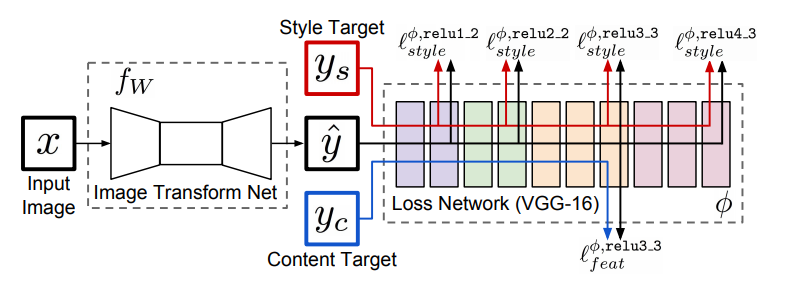
After training, we can use that network for styling any image in one pass without the need of optimization
The main highlights of the network:
- Residual Layers
- Encoder-Decoder Model
- output from decoder is passed to loss model(VGG) to calculate the loss
- training needs compute as we are passing these images to two networks on every step
Define loss
For calculating style loss and content loss we need a pre-trained model, we are using vgg19 the original implementation uses vgg16.
1
2
vgg=vgg19.VGG19(weights='imagenet',include_top=False)
vgg.summary()
Model: "vgg19"
_________________________________________________________________
Layer (type)                 Output Shape              Param #
=================================================================
input_1 (InputLayer)         [(None, None, None, 3)]   0
_________________________________________________________________
block1_conv1 (Conv2D)        (None, None, None, 64)    1792
_________________________________________________________________
block1_conv2 (Conv2D)        (None, None, None, 64)    36928
_________________________________________________________________
block1_pool (MaxPooling2D)   (None, None, None, 64)    0
_________________________________________________________________
block2_conv1 (Conv2D)        (None, None, None, 128)   73856
_________________________________________________________________
block2_conv2 (Conv2D)        (None, None, None, 128)   147584
_________________________________________________________________
block2_pool (MaxPooling2D)   (None, None, None, 128)   0
_________________________________________________________________
block3_conv1 (Conv2D)        (None, None, None, 256)   295168
_________________________________________________________________
block3_conv2 (Conv2D)        (None, None, None, 256)   590080
_________________________________________________________________
block3_conv3 (Conv2D)        (None, None, None, 256)   590080
_________________________________________________________________
block3_conv4 (Conv2D)        (None, None, None, 256)   590080
_________________________________________________________________
block3_pool (MaxPooling2D)   (None, None, None, 256)   0
_________________________________________________________________
block4_conv1 (Conv2D)        (None, None, None, 512)   1180160
_________________________________________________________________
block4_conv2 (Conv2D)        (None, None, None, 512)   2359808
_________________________________________________________________
block4_conv3 (Conv2D)        (None, None, None, 512)   2359808
_________________________________________________________________
block4_conv4 (Conv2D)        (None, None, None, 512)   2359808
_________________________________________________________________
block4_pool (MaxPooling2D)   (None, None, None, 512)   0
_________________________________________________________________
block5_conv1 (Conv2D)        (None, None, None, 512)   2359808
_________________________________________________________________
block5_conv2 (Conv2D)        (None, None, None, 512)   2359808
_________________________________________________________________
block5_conv3 (Conv2D)        (None, None, None, 512)   2359808
_________________________________________________________________
block5_conv4 (Conv2D)        (None, None, None, 512)   2359808
_________________________________________________________________
block5_pool (MaxPooling2D)   (None, None, None, 512)   0
=================================================================
Total params: 20,024,384
Trainable params: 20,024,384
Non-trainable params: 0
_________________________________________________________________
Here we define layers that we will use to calculate the loss.
1
2
3
4
5
6
7
content_layers=['block4_conv2']

style_layers=['block1_conv1',
            'block2_conv1',
            'block3_conv1',
            'block4_conv1',
            'block5_conv1']
Let’s define a class that creates a loss model with some additional methods for accessing feature maps from the network. We have also used these functions in the previous post, here we just encapsulated them inside a class.
1
2
3
4
5
6
7
8
9
10
11
12
13
14
15
16
17
18
19
20
21
22
class LossModel:
    def __init__(self,pretrained_model,content_layers,style_layers):
        self.model=pretrained_model
        self.content_layers=content_layers
        self.style_layers=style_layers
        self.loss_model=self.get_model()

    def get_model(self):
        self.model.trainable=False
        layer_names=self.style_layers + self.content_layers
        outputs=[self.model.get_layer(name).output for name in layer_names]
        new_model=Model(inputs=self.model.input,outputs=outputs)
        return new_model

    def get_activations(self,inputs):
        inputs=inputs*255.0
        style_length=len(self.style_layers)
        outputs=self.loss_model(vgg19.preprocess_input(inputs))
        style_output,content_output=outputs[:style_length],outputs[style_length:]
        content_dict={name:value for name,value in zip(self.content_layers,content_output)}
        style_dict={name:value for name,value in zip(self.style_layers,style_output)}
        return {'content':content_dict,'style':style_dict}
Now we create our loss model using the above class
1
loss_model = LossModel(vgg, content_layers, style_layers)
Let us define loss function for calculating content and style loss, below methods content_loss and style _loss calculates content and style loss respectively. With weighted averaging of these losses, we derive perceptual loss defined in preceptual_loss function. The details of these loss functions are covered in the previous post.
1
2
3
def content_loss(placeholder,content,weight):
    assert placeholder.shape == content.shape
    return weight*tf.reduce_mean(tf.square(placeholder-content))
1
2
3
def gram_matrix(x):
    gram=tf.linalg.einsum('bijc,bijd->bcd', x, x)
    return gram/tf.cast(x.shape[1]*x.shape[2]*x.shape[3],tf.float32)
1
2
3
4
5
def style_loss(placeholder,style, weight):
    assert placeholder.shape == style.shape
    s=gram_matrix(style)
    p=gram_matrix(placeholder)
    return weight*tf.reduce_mean(tf.square(s-p))
1
2
3
4
5
6
7
8
9
10
11
12
def preceptual_loss(predicted_activations,content_activations,
                    style_activations,content_weight,style_weight,
                    content_layers_weights,style_layer_weights):
    pred_content = predicted_activations["content"]
    pred_style = predicted_activations["style"]
    c_loss = tf.add_n([content_loss(pred_content[name],content_activations[name],
                                  content_layers_weights[i]) for i,name in enumerate(pred_content.keys())])
    c_loss = c_loss*content_weight
    s_loss = tf.add_n([style_loss(pred_style[name],style_activations[name],
                                style_layer_weights[i]) for i,name in enumerate(pred_style.keys())])
    s_loss = s_loss*style_weight
    return c_loss+s_loss
Create an Autoencoder
Here we first defined all necessary layers for our network:
ReflectionPadding2D: for applying reflection padding to images in conv netsInstanceNormalization: We are using instance normalization instead of batch normalization as it gives a better result. It normalizes inputs across the channel.ConvLayer: Block of conv layer with padding-> conv_layer-> instance_normalization combinedResidualLayer: Residual layer with two ConvLayer blockUpsampleLayer: upsample the bottleneck representation (if you have read about autoencoders you know what I mean) in autoencoder. It can be considered as deconvolutional layers.
1
2
3
4
5
6
7
8
class ReflectionPadding2D(tf.keras.layers.Layer):
    def __init__(self, padding=(1, 1), **kwargs):
        super(ReflectionPadding2D, self).__init__(**kwargs)
        self.padding = tuple(padding)
    def call(self, input_tensor):
        padding_width, padding_height = self.padding
        return tf.pad(input_tensor, [[0,0], [padding_height, padding_height],
                                     [padding_width, padding_width], [0,0] ], 'REFLECT')
1
2
3
4
5
6
7
8
9
10
11
class InstanceNormalization(tf.keras.layers.Layer):
    def __init__(self,**kwargs):
        super(InstanceNormalization, self).__init__(**kwargs)
    def call(self,inputs):
        batch, rows, cols, channels = [i for i in inputs.get_shape()]
        mu, var = tf.nn.moments(inputs, [1,2], keepdims=True)
        shift = tf.Variable(tf.zeros([channels]))
        scale = tf.Variable(tf.ones([channels]))
        epsilon = 1e-3
        normalized = (inputs-mu)/tf.sqrt(var + epsilon)
        return scale * normalized + shift
1
2
3
4
5
6
7
8
9
10
11
class ConvLayer(tf.keras.layers.Layer):
    def __init__(self,filters,kernel_size,strides=1,**kwargs):
        super(ConvLayer,self).__init__(**kwargs)
        self.padding=ReflectionPadding2D([k//2 for k in kernel_size])
        self.conv2d=tf.keras.layers.Conv2D(filters,kernel_size,strides)
        self.bn=InstanceNormalization()
    def call(self,inputs):
        x=self.padding(inputs)
        x=self.conv2d(x)
        x=self.bn(x)
        return x
1
2
3
4
5
6
7
8
9
10
11
12
13
14
class ResidualLayer(tf.keras.layers.Layer):
    def __init__(self,filters,kernel_size,**kwargs):
        super(ResidualLayer,self).__init__(**kwargs)
        self.conv2d_1=ConvLayer(filters,kernel_size)
        self.conv2d_2=ConvLayer(filters,kernel_size)
        self.relu=tf.keras.layers.ReLU()
        self.add=tf.keras.layers.Add()
    def call(self,inputs):
        residual=inputs
        x=self.conv2d_1(inputs)
        x=self.relu(x)
        x=self.conv2d_2(x)
        x=self.add([x,residual])
        return x
1
2
3
4
5
6
7
8
9
10
11
12
class UpsampleLayer(tf.keras.layers.Layer):
    def __init__(self,filters,kernel_size,strides=1,upsample=2,**kwargs):
        super(UpsampleLayer,self).__init__(**kwargs)
        self.upsample=tf.keras.layers.UpSampling2D(size=upsample)
        self.padding=ReflectionPadding2D([k//2 for k in kernel_size])
        self.conv2d=tf.keras.layers.Conv2D(filters,kernel_size,strides)
        self.bn=InstanceNormalization()
    def call(self,inputs):
        x=self.upsample(inputs)
        x=self.padding(x)
        x=self.conv2d(x)
        return self.bn(x)
Using these layers defined above let’s create a convolutional autoencoder.
Architecture:
- 3 X ConvLayer
- 5 X ResidualLayer
- 3 X UpsampleLayer
1
2
3
4
5
6
7
8
9
10
11
12
13
14
15
16
17
18
19
20
21
22
23
24
25
26
27
28
29
30
31
32
33
34
35
36
37
38
39
40
41
42
43
44
45
46
47
48
49
50
51
52
53
54
55
56
57
58
59
60
61
62
63
64
65
66
class StyleTransferModel(tf.keras.Model):
    def __init__(self,**kwargs):
        super(StyleTransferModel, self).__init__(name='StyleTransferModel',**kwargs)
        self.conv2d_1= ConvLayer(filters=32,kernel_size=(9,9),strides=1,name="conv2d_1_32")
        self.conv2d_2= ConvLayer(filters=64,kernel_size=(3,3),strides=2,name="conv2d_2_64")
        self.conv2d_3= ConvLayer(filters=128,kernel_size=(3,3),strides=2,name="conv2d_3_128")
        self.res_1=ResidualLayer(filters=128,kernel_size=(3,3),name="res_1_128")
        self.res_2=ResidualLayer(filters=128,kernel_size=(3,3),name="res_2_128")
        self.res_3=ResidualLayer(filters=128,kernel_size=(3,3),name="res_3_128")
        self.res_4=ResidualLayer(filters=128,kernel_size=(3,3),name="res_4_128")
        self.res_5=ResidualLayer(filters=128,kernel_size=(3,3),name="res_5_128")
        self.deconv2d_1= UpsampleLayer(filters=64,kernel_size=(3,3),name="deconv2d_1_64")
        self.deconv2d_2= UpsampleLayer(filters=32,kernel_size=(3,3),name="deconv2d_2_32")
        self.deconv2d_3= ConvLayer(filters=3,kernel_size=(9,9),strides=1,name="deconv2d_3_3")
        self.relu=tf.keras.layers.ReLU()
    def call(self, inputs):
        x=self.conv2d_1(inputs)
        x=self.relu(x)
        x=self.conv2d_2(x)
        x=self.relu(x)
        x=self.conv2d_3(x)
        x=self.relu(x)
        x=self.res_1(x)
        x=self.res_2(x)
        x=self.res_3(x)
        x=self.res_4(x)
        x=self.res_5(x)
        x=self.deconv2d_1(x)
        x=self.relu(x)
        x=self.deconv2d_2(x)
        x=self.relu(x)
        x=self.deconv2d_3(x)
        x = (tf.nn.tanh(x) + 1) * (255.0 / 2)
        return x

    ## used to print shapes of each layer to check if input shape == output shape
    ## I don't know any better solution to this right now
    def print_shape(self,inputs):
        print(inputs.shape)
        x=self.conv2d_1(inputs)
        print(x.shape)
        x=self.relu(x)
        x=self.conv2d_2(x)
        print(x.shape)
        x=self.relu(x)
        x=self.conv2d_3(x)
        print(x.shape)
        x=self.relu(x)
        x=self.res_1(x)
        print(x.shape)
        x=self.res_2(x)
        print(x.shape)
        x=self.res_3(x)
        print(x.shape)
        x=self.res_4(x)
        print(x.shape)
        x=self.res_5(x)
        print(x.shape)
        x=self.deconv2d_1(x)
        print(x.shape)
        x=self.relu(x)
        x=self.deconv2d_2(x)
        print(x.shape)
        x=self.relu(x)
        x=self.deconv2d_3(x)
        print(x.shape)
define input shape and batch_size here
1
2
input_shape=(256,256,3)
batch_size=4
Create style model using StyleTransferModel class
1
style_model = StyleTransferModel()
Here we check the shape of all layers and verify input shape and output shape
1
style_model.print_shape(tf.zeros(shape=(1,*input_shape)))
(1, 256, 256, 3)
(1, 256, 256, 32)
(1, 128, 128, 64)
(1, 64, 64, 128)
(1, 64, 64, 128)
(1, 64, 64, 128)
(1, 64, 64, 128)
(1, 64, 64, 128)
(1, 64, 64, 128)
(1, 128, 128, 64)
(1, 256, 256, 32)
(1, 256, 256, 3)
Training model
Here we have defined an optimizer for training, we are using Adam optimizer with learning rate 1e-3
1
optimizer = tf.keras.optimizers.Adam(learning_rate=1e-3)
1
2
3
4
5
6
7
8
9
10
11
12
13
14
15
16
17
18
19
20
21
22
23
24
25
26
27
def train_step(dataset,style_activations,steps_per_epoch,style_model,loss_model,optimizer,
               checkpoint_path="./",content_weight=1e4, style_weight=1e-2,
               total_variation_weight=0.004):
    batch_losses=[]
    steps=1
    save_path=os.path.join(checkpoint_path,f"model_checkpoint.ckpt")
    print("Model Checkpoint Path: ",save_path)
    for input_image_batch in dataset:
        if steps-1 >= steps_per_epoch:
            break
        with tf.GradientTape() as tape:
            outputs=style_model(input_image_batch)
            outputs=tf.clip_by_value(outputs, 0, 255)
            pred_activations=loss_model.get_activations(outputs/255.0)
            content_activations=loss_model.get_activations[input_image_batch]("content")
            curr_loss=preceptual_loss(pred_activations,content_activations,style_activations,content_weight,
                                      style_weight,content_layers_weights,style_layers_weights)
            curr_loss += total_variation_weight*tf.image.total_variation(outputs)
        batch_losses.append(curr_loss)
        grad = tape.gradient(curr_loss,style_model.trainable_variables)
        optimizer.apply_gradients(zip(grad,style_model.trainable_variables))
        if steps % 1000==0:
            print("checkpoint saved ",end=" ")
            style_model.save_weights(save_path)
            print(f"Loss: {tf.reduce_mean(batch_losses).numpy()}")
        steps+=1
    return tf.reduce_mean(batch_losses)
In the above function, we have defined a single training step. Inside the function:
- first, we defined save_path for model checkpointing
- for number of steps_per_epoch we run a training loop
- for every step, we forward pass a batch of image pass it to our loss model
- get content_layer activations for the batch of images
- together with style activations from style image and content activations we calculate the perceptual loss
- we add some total variation loss to image for smoothening
- calculate gradients of the loss function with respect to the model’s trainable parameters
- finally backpropagates to optimize
- at every 1000 steps saving checkpoints
Configure Dataset for training
Downloading coco dataset for training, we can use any other image dataset with images in bulk. Below line downloads coco dataset using wget in zip format. Further, we create a directory where we unzip that downloaded zip file.
1
wget <http://images.cocodataset.org/zips/train2014.zip>
--2020-07-12 08:14:59--  http://images.cocodataset.org/zips/train2014.zip
Resolving images.cocodataset.org (images.cocodataset.org)... 52.216.224.88
Connecting to images.cocodataset.org (images.cocodataset.org)|52.216.224.88|:80... connected.
HTTP request sent, awaiting response... 200 OK
Length: 13510573713 (13G) [application/zip]
Saving to: ‘train2014.zip’

train2014.zip       100%[===================>]  12.58G  25.0MB/s    in 6m 56s

2020-07-12 08:21:55 (31.0 MB/s) - ‘train2014.zip’ saved [13510573713/13510573713]
1
2
mkdir coco
unzip -qq train2014.zip -d coco
For training, the model lets create tensorflow dataset which loads all images from the path specified resize them to be of the same size for efficient batch training and implements batching and prefetching. Below class creates tfdataset for training.
Note we are training model with fixed-size images but we can generate images of any size because all layers in model are convolutional layers.
1
2
3
4
5
6
7
8
9
10
11
12
13
14
15
16
17
18
19
20
21
22
23
class TensorflowDatasetLoader:
    def __init__(self,dataset_path,batch_size=4, image_size=(256, 256),num_images=None):
        images_paths = [str(path) for path in Path(dataset_path).glob("*.jpg")]
        self.length=len(images_paths)
        if num_images is not None:
            images_paths = images_paths[0:num_images]
        dataset = tf.data.Dataset.from_tensor_slices(images_paths).map(
            lambda path: self.load_tf_image(path, dim=image_size),
            num_parallel_calls=tf.data.experimental.AUTOTUNE,
        )
        dataset = dataset.batch(batch_size,drop_remainder=True)
        dataset = dataset.repeat()
        dataset = dataset.prefetch(buffer_size=tf.data.experimental.AUTOTUNE)
        self.dataset=dataset
    def __len__(self):
        return self.length
    def load_tf_image(self,image_path,dim):
        image = tf.io.read_file(image_path)
        image = tf.image.decode_jpeg(image, channels=3)
        image= tf.image.resize(image,dim)
        image= image/255.0
        image = tf.image.convert_image_dtype(image, tf.float32)
        return image
using the above class lets create tfdataset from coco dataset images. We specify the path to images folder (where all images reside) and batch size
1
loader=TensorflowDatasetLoader("coco/train2014/",batch_size=4)
1
loader.dataset.element_spec
TensorSpec(shape=(4, 256, 256, 3), dtype=tf.float32, name=None)
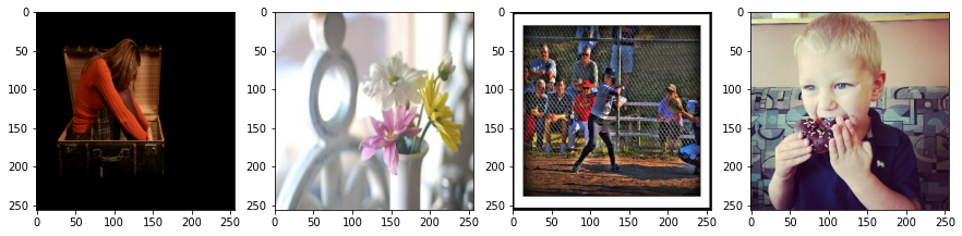
plot some images to see how images in dataset looks
1
plot_images_grid(next(iter(loader.dataset.take(1))))
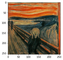
Now lets load style image from URL using load_url_image and plot it.
1
2
3
4
5
# setting up style image

url="https://www.edvardmunch.org/images/paintings/the-scream.jpg"
style_image=load_url_image(url,dim=(input_shape[0],input_shape[1]),resize=True)
style_image=style_image/255.0
1
show_image(style_image)
Next, we extract style layers feature maps of style image using loss model
1
2
3
style_image=style_image.astype(np.float32)
style_image_batch=np.repeat([style_image],batch_size,axis=0)
style_activations=loss_model.get_activations[style_image_batch]("style")
Training model
define content weight, style weight and total variation weight these are hyperparameters which we can tune to change the strength of style and content in the output image
1
2
3
content_weight=1e1
style_weight=1e2
total_variation_weight=0.004
Now define the number of epochs to train, steps per epochs and model checkpoint path
1
epochs=2
1
2
3
num_images=len(loader)
steps_per_epochs=num_images//batch_size
print(steps_per_epochs)
20695
1
save_path = "./scream"
1
os.makedirs(save_path, exist_ok=True)
Enable mixed-precision training it offers significant computational speedup by performing operations in half-precision format.
1
2
3
4
5
try:
    policy = tf.keras.mixed_precision.experimental.Policy('mixed_float16')
    tf.keras.mixed_precision.experimental.set_policy(policy)
except:
    pass
if the previous checkpoint exists at that path load that checkpoint and continue further training else we train from scratch
1
2
3
4
5
if os.path.isfile(os.path.join(save_path,"model_checkpoint.ckpt.index")):
    style_model.load_weights(os.path.join(save_path,"model_checkpoint.ckpt"))
    print("resuming training ...")
else:
    print("training scratch ...")
training scratch ...
Finally, we start training the model. At each epoch, we are calling train_step function which runs till number of steps per epochs defined and after every epoch save model checkpoint for further inferencing and training.
1
2
3
4
5
6
7
8
9
10
11
epoch_losses=[]
for epoch in range(1,epochs+1):
    print(f"epoch: {epoch}")
    batch_loss=train_step(loader.dataset,style_activations,steps_per_epochs,style_model,loss_model,optimizer,
                          save_path,
                          content_weight,style_weight,total_variation_weight,
                          content_layers_weights,style_layers_weights)
    style_model.save_weights(os.path.join(save_path,"model_checkpoint.ckpt"))
    print("Model Checkpointed at: ",os.path.join(save_path,"model_checkpoint.ckpt"))
    print(f"loss: {batch_loss.numpy()}")
    epoch_losses.append(batch_loss)
epoch: 1
Model Checkpoint Path:  ./scream/model_checkpoint.ckpt
checkpoint saved  Loss: 6567731.5
checkpoint saved  Loss: 6464426.5
checkpoint saved  Loss: 6402768.0
checkpoint saved  Loss: 6336974.5
checkpoint saved  Loss: 6281922.5
checkpoint saved  Loss: 6232056.0
checkpoint saved  Loss: 6191586.5
checkpoint saved  Loss: 6155332.0
checkpoint saved  Loss: 6119712.5
checkpoint saved  Loss: 6085571.5
checkpoint saved  Loss: 6062698.0
checkpoint saved  Loss: 6036787.0
checkpoint saved  Loss: 6011265.5
checkpoint saved  Loss: 5988809.5
checkpoint saved  Loss: 5969908.0
checkpoint saved  Loss: 5950925.0
checkpoint saved  Loss: 5931179.5
checkpoint saved  Loss: 5912791.5
checkpoint saved  Loss: 5894602.0
checkpoint saved  Loss: 5880713.0
Model Checkpointed at:  ./scream
loss: 5869695.5
epoch: 2
Model Checkpoint Path:  ./scream/model_checkpoint.ckpt
checkpoint saved  Loss: 5520494.5
checkpoint saved  Loss: 5532450.5
checkpoint saved  Loss: 5529669.0
checkpoint saved  Loss: 5524684.0
checkpoint saved  Loss: 5518524.5
checkpoint saved  Loss: 5508913.5
checkpoint saved  Loss: 5503493.5
checkpoint saved  Loss: 5501864.0
checkpoint saved  Loss: 5497016.0
checkpoint saved  Loss: 5491713.0
checkpoint saved  Loss: 5491244.5
checkpoint saved  Loss: 5484620.0
checkpoint saved  Loss: 5482881.0
checkpoint saved  Loss: 5476766.5
checkpoint saved  Loss: 5472491.0
checkpoint saved  Loss: 5466294.5
checkpoint saved  Loss: 5459984.0
checkpoint saved  Loss: 5454912.5
checkpoint saved  Loss: 5449535.5
checkpoint saved  Loss: 5446370.0
Model Checkpointed at:  ./scream
loss: 5442546.5
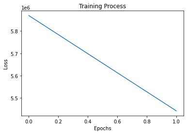
After training model lets plot loss concerning epochs and check loss summary
1
2
3
4
5
plt.plot(epoch_losses)
plt.xlabel("Epochs")
plt.ylabel("Loss")
plt.title("Training Process")
plt.show()
Now its time to generate some style images. We start first by loading the saved model checkpoint into autoencoder.
1
2
3
4
5
if os.path.isfile(os.path.join(save_path,"model_checkpoint.ckpt.index")):
    style_model.load_weights(os.path.join(save_path,"model_checkpoint.ckpt"))
    print("loading weights ...")
else:
    print("no weights found ...")
loading weights ...
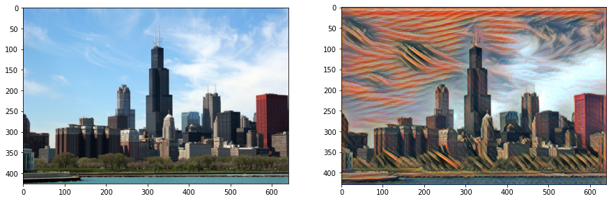
load an image for styling and convert it to float.
1
test_image_url="https://hips.hearstapps.com/hmg-prod.s3.amazonaws.com/images/chicago-skyline-on-a-clear-day-royalty-free-image-115891582-1557159569.jpg"
1
2
test_image=load_url_image(test_image_url,dim=(640,480))
test_image=np.expand_dims(test_image,axis=0)
1
test_image=test_image.astype(np.float32)
In one forward pass of the model, we get generated styled image
1
predicted_image=style_model(test_image)
Clamp generated image pixels between 0 to 255 and convert it to uint8. We got our generated style image, plot it and check how its looks also save it and share with friends
1
2
predicted_image=np.clip(predicted_image,0,255)
predicted_image=predicted_image.astype(np.uint8)
1
2
3
test_output=test_image.astype(np.uint8)
test_output=tf.squeeze(test_output).numpy()
predicted_output=tf.squeeze(predicted_image).numpy()
1
plot_images_grid([test_output,predicted_output])
If you do not have enough compute power use colab or kaggle kernels they provide free GPU even TPU for training these models, Once trained we can use trained checkpoints to do style transfer in any system with GPU or CPU.
Using opencv we can easily create styled videos too.
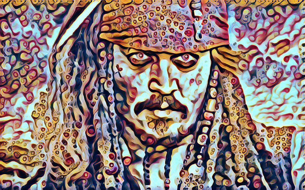
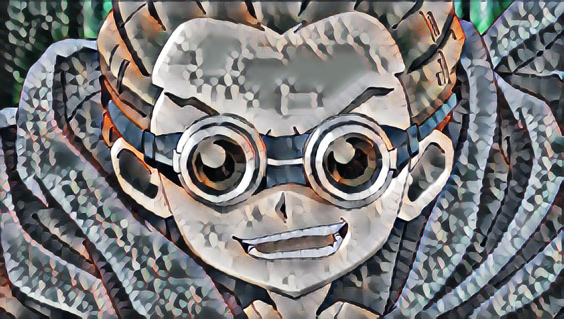
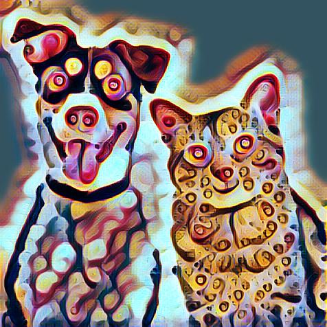
Results
Some Image results

Here we have realtime video stylization in action
Below is a youtube video which shows video stylization in action

Now generate different images and videos, play with it and share exciting results.
If someone wants to try style transfer in video and images right now, I have created a github repository for the same purpose with instructions.
Thanks for reading. ✌✌✌
References
- Instance Normalization: The Missing Ingredient for Fast Stylization
- Perceptual Losses for Real-Time Style Transfer and Super-Resolution
- A Neural Algorithm of Artistic Style