introduction to deep learning and perceptron

Deep Learning is subset of machine learning which on its own subset of Artificial Intelligence, that has seen boom after 2012 with the increase in amount of data and compute (especially with introduction of GPU for deep learning). Now these networks are part of our daily life. Google searches, Google translate, ChatGPT, Image processing etc. are few examples that uses deep learning in their backend. Like machine learning we learn rules from data, instead of hand code rules to program we make algorithm learn those rule. Deep learning emphasis on learning representations from data in hierarchical manner which is inspired from brain, where subsequent layers learns different features. Deep Learning is different from classical machine learning as it can learn from unstructured data like images, audio, texts etc. while in classical machine learning we have to specifically encode these to some representations that then can be fed to machine learning algorithm, but for deep learning they learn on its own. Example: haar cascade face detection algorithm uses set of cleverly designed features from faces and then these features are put into ML algorithm (SVM). While deep learning will take image as input and learn from that, so no need to design features they will learn those.

History

• It originated from the field which now known as cybernetics
• 1940 : McCulloch and Pitts came up with idea of neurons as threshold unit with on/off states.
• 1947: Donal Hebb proposed that neuron in brain learn by modifying strength of the connections between neurons.
• 1957: Frank Rosenblatt proposed Perceptron
• took off in 1950’s and died in 1960’s
• Failed because, researchers used binary neurons, also multiplication is very costly operation at that time.
• took off again in 1985 with emergence of backpropagation
• 1995: again died, dominance of SVM.
• 2010: neural network shows huge performance in speech recognition systems.
• 2012: Alexnet shows huge performance boost in Imagenet data.
• 2013: computer vision shifted to neural networks
• 2016: NLP community also shifts to neural nets.
• present: many AI trends like generating modalities (DALLE, GPT), robotics, control, games (Dota2, Alphago) use neural nets.

SUMMARY: Deep Learning is subset of Machine Learning which itself is subset of AI. It is different from ML, as it can learn from unstructured data and discover patterns from data without explicitly defined features. It is widely used currently because of availability of large volumes of data and computation power.

Perceptron

• It is a simple machine learning algorithm inspired from working of human brain later which gave rise to modern neural networks.

• F. Rosenblatt gave the idea of perceptron in his paper titled The Perceptron: A Probabilistic model for information storage and organization in the brain.

• It assumes that similar stimuli create connections with the same set of cells, while dissimilar stimuli create connections with different sets of cells in the brain.

• It can be thought as a function that takes some input process it and provide some output.

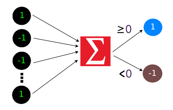
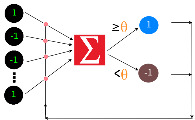
• It was introduced as classification model, it assumes a constant value \(\theta\) called threshold. If output lies above this threshold it gives 1 else -1

• It learns from feedback provided when the prediction given by it is wrong.

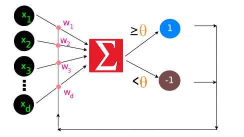
• Input given is of form \(x = (x_1, x_2, ……, x_n) \in \mathbb{R}^d\).

• weight vectors are associated to each connections. \(w = (w_1, w_2, ….., w_d) \in \mathbb{R}^d\)

Perceptron Prediction Rule

• \(\sum_\limits{i=1}^\limits{d} w_ix_i = \langle w,x \rangle\) is dot product of weight vector with input vector.

we can also write above equations as

we can incorporate \(\theta\) inside \(w\) as \(w_0\) and append \(x\) with \(1\), to make equation as

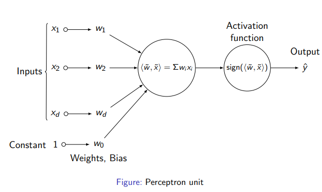
Geometric Intuition

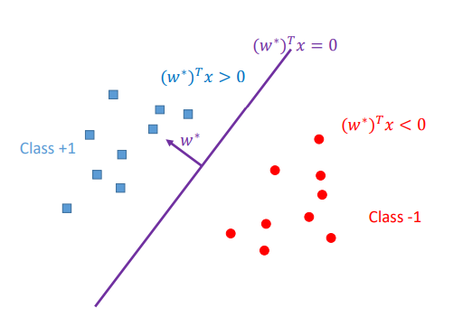
• \(w\) can be seen as vector representing hyperplane, which is perpendicular to that hyperplane.

• Equation of hyperplane is \(w^T + b = 0\) where \(w \in \mathbb{R}^d\) and \(b\) is intercept term, also vector \(w\) is perpendicular to hyperplane.

• For geometric intuition of perceptron we can thought vector \(w\) corresponding to a hyperplane that divides data into two classes.

• When learning we will learn optimal value of \(w\) such that hyperplane corresponding divides data into two classes.

• Using prediction rule we can find which class new point \(x_{new}\) belongs \(\langle w, x_{new} \rangle\) and check which side of hyperplane this new point lies.

Perceptron Update Rule

Algorithm

• Initialize weight vector with \(0\) ie.. \(w_i = 0 \ \ \forall \ i=1, ..., d\) and initialize \(t = 1\)
• Given an example \(x\), predict \(1\) iff \(w^t \cdot x > 0\) else predict \(-1\)
• On a mistake, update \(w^{t+1} \leftarrow w^t + y^tx^t\).
• \(t \leftarrow t+1\).

We only update perceptron weights only when mistake occurs using the update rule \(w^{t+1} = w^t + y^tx^t\).

Code Implementation

Import required packages

1
2
3
import numpy as np
import matplotlib.pyplot as plt
import random

1
2
3
# seed random number generator of numpy for reproducibility

np.random.seed(1000)

Data Generation

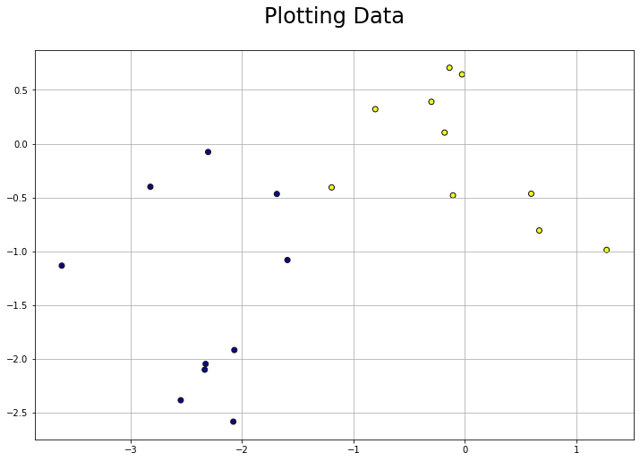
Generating \(10\) two-dimensional data points from a multi-variate Gaussian distribution with mean \([0,0]\) and identity covariance matrix and label them as \(+1\).

1
2
3
4
5
6
7
8
9
10
11
12
13
14
15
16
17
18
# Generate data with mean [0,0] and identity covariance matrix

size = 10
identity_matrix = [[1, 0],
                   [0, 1]]

# features

x = np.random.multivariate_normal(mean=[0, 0], cov=identity_matrix, size=size)

# label all points as +1

y = np.array([1]*size)

# full data with label +1

d1 = np.concatenate([x, np.expand_dims(y, axis=1)], axis=1)
print(d1.shape)

(10, 3)

Generating \(10\) two-dimensional data points from a multi-variate Gaussian distribution with mean \([-2,-2]\) and identity covariance matrix and label them as \(-1\).

1
2
3
4
5
6
7
8
9
10
11
12
13
14
15
16
17
18
19
# Generate data with mean [-2, -2] and identity covariance matrix.

size = 10
identity_matrix = [[1, 0],
                   [0, 1]]

# features

x = np.random.multivariate_normal(mean=[-2, -2], cov=identity_matrix, size=size)

# labels all points as -1

y = np.array([-1]\*size)

# full data with label -1

d2 = np.concatenate([x, np.expand_dims(y, axis=1)], axis=1)

print(d2.shape)

(10, 3)

1
2
3
4
5
6
7
8
9
10
11
# Construct dataset D and shuffle.

# concatenate data into d

d = np.concatenate([d1, d2], axis=0)

# shuffle data

np.random.shuffle(d)

print(d.shape)

(20, 3)

Data Visualization

Function to visualize the dataset.

1
2
3
4
5
6
7
8
def plot_data(data):
features = data[:, :-1]
labels = data[:, -1]
plt.figure(figsize=(12, 8))
plt.scatter(x=features[:, 0], y=features[:, 1], c=labels, cmap="plasma", edgecolors="#111")
plt.grid()
plt.title("Plotting Data", pad=30, fontdict={"fontsize": 24})
plt.show()

1
plot_data(d)

Perceptron prediction rule

1
2
3
4
def activation(out):
if out >=0:
return 1
return -1

1
2
3
def perceptron_prediction(w, x): # compute the prediction for the example x using weight w
out = np.dot(w, x)
return activation(out)

Perceptron update rule

1
2
3
4
5
6
def perceptron_update_weights(w, x, y, y_pred):
is_mistake = False # check for mistake and set is_mistake flag accordingly
if y != y_pred:
is_mistake = True # and write code to update the weights in perceptron
w = w + x\*y
return w, is_mistake

Training procedure for perceptron

This function takes data and trains the perceptron to classify the datapoints into appropriate classes.

1
2
3
4
5
6
7
8
9
10
11
12
13
14
15
16
17
18
19
20
21
22
23
24
25
26
27
def train_perceptron(data): # Initialize weights
w = np.zeros(shape=(3, )) # we can also initialize with random weights # w = np.random.normal(size=(3, ))
epochs = 0
num_mistakes = 99
max_epochs = 50

while num_mistakes > 0 and epochs<max_epochs:
num_mistakes = 0
for i in range(len(data)): # retrieve the feature vector x from data set D
x = data[i, :-1]

      # Append an additional constant feature 1 to x
      x = np.concatenate([x, [1]])

      y_hat = perceptron_prediction(w, x)

      # retrieve the label y for x from data set D
      y = data[i, -1]

      w, is_mistake = perceptron_update_weights(w, x, y, y_hat)

      if is_mistake:
        num_mistakes += 1
    print(f"Epoch {epochs+1} completed, Number of mistakes: {num_mistakes}")
    epochs=epochs+1

return w

1
w_final = train_perceptron(d)

Epoch 1 completed, Number of mistakes: 5
Epoch 2 completed, Number of mistakes: 3
Epoch 3 completed, Number of mistakes: 2
Epoch 4 completed, Number of mistakes: 1
Epoch 5 completed, Number of mistakes: 0

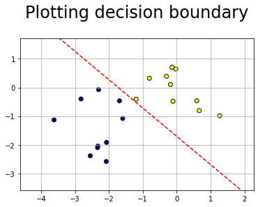
Plotting the decision boundary (seperating line)

1
2
3
4
5
6
7
8
def plot_line(w, xlim=None):
axes = plt.gca()

# get x limits

x_vals = np.array(axes.get_xlim())
y_vals = -(w[2] + w[0] \* x_vals)/w[1]
plt.plot(x_vals, y_vals, 'r--')

1
2
3
4
5
6
7
8
9
10
def plot_data_with_separator(data, w):
features = data[:, :-1]
labels = data[:, -1]
plt.scatter(x=features[:, 0], y=features[:, 1], c=labels, cmap="plasma", edgecolors="#111")
plt.xlim([features[:, 0].min() - 1, features[:, 0].max() + 1])
plt.ylim([features[:, 1].min() - 1, features[:, 1].max() + 1])
plot_line(w)
plt.grid()
plt.title("Plotting decision boundary", pad=30, fontdict={"fontsize": 24})
plt.show()

1
plot_data_with_separator(d, w_final)

Lets also animate each perceptron update step

1
!pip install -qq ffmpeg-python

1
2
from matplotlib.animation import FuncAnimation
from IPython.display import HTML

1
2
3
4
5
6
7
8
9
10
11
12
13
14
15
16
17
18
19
20
21
22
23
24
25
26
27
28
29
30
31
32
33
34
35
36
37
38
39
40
41
42
weights = np.zeros(shape=(3,))
data = d
epochs = 0
features = data[:, :-1]
labels = data[:, -1]

fig, ax = plt.subplots(figsize=(12, 8))
ax.grid()
ax.scatter(x=features[:, 0], y=features[:, 1], c=labels, cmap="plasma", edgecolors="#111")
ax.set_xlim([features[:, 0].min() - 1, features[:, 0].max() + 1])
ax.set_ylim([features[:, 1].min() - 1, features[:, 1].max() + 1])
line, = ax.plot([], [], 'r', lw=2)
ax.set_title("Plot Data", pad=30, fontdict={"fontsize": 24})
x_vals = np.array(ax.get_xlim())
plt.close()

def animation(i):
global weights
ax.set_title(f"Plotting decision boundary, dataset iteration: {i+1}", pad=30, fontdict={"fontsize": 24})
if weights[1] == 0: # for solving divide by zero error
y_vals = -(weights[2] + weights[0] * x*vals)
else:
y_vals = -(weights[2] + weights[0] \* x_vals)/weights[1]
line.set_data(x_vals, y_vals)

    # retrieve the feature vector x from data set D

    x = data[i, :-1]

    # Append an additional constant feature 1 to x (Use np.concatenate)

    x = np.concatenate([x, [1]])

    y_hat = perceptron_prediction(weights, x)

    # retrieve the label y for x from data set D

    y = data[i, -1]

    weights, is_mistake = perceptron_update_weights(weights, x, y, y_hat)

return line,

1
2
3
4
epochs += 1
print("Video Epoch ", epochs)
anim = FuncAnimation(fig, animation, frames=len(data), interval=500, blit=True)
HTML(anim.to_html5_video())

Video Epoch 1

Video Link

1
2
3
4
epochs += 1
print("Video Epoch ", epochs)
anim = FuncAnimation(fig, animation, frames=len(data), interval=500, blit=True)
HTML(anim.to_html5_video())

Video Epoch 2

Video Link

1
2
3
4
epochs += 1
print("Video Epoch ", epochs)
anim = FuncAnimation(fig, animation, frames=len(data), interval=500, blit=True)
HTML(anim.to_html5_video())

Video Epoch 3

Video Link

1
2
3
4
epochs += 1
print("Video Epoch ", epochs)
anim = FuncAnimation(fig, animation, frames=len(data), interval=500, blit=True)
HTML(anim.to_html5_video())

Video Epoch 4

Video Link

1
2
3
4
epochs += 1
print("Video Epoch ", epochs)
anim = FuncAnimation(fig, animation, frames=len(data), interval=500, blit=True)
HTML(anim.to_html5_video())

Video Epoch 5

Video Link

Perceptron Convergence Theorem

For any finite set of linearly separable labeled examples, the Perceptron Learning Algorithm will halt after a finite number of iterations.

• Under linear seperable assumptions of positive and negative samples the training procedure for perceptron converges in finite time.

• Linear seperability means there exist a hyperplane \(w^*\)such that it divides data into two seperate regions.

for some \(\gamma > 0\) where \(\gamma\) is margin, which is minimum distance of data points from seperating hyperplane.

Perceptron is said to be converged when in has learned the seperating hyperplane between data points ie. points that are false classified is none, or mistake \(= 0\). If we can find the bounds of number of mistakes, which will denote that perceptron can do atmost these number of mistakes then we have also proved that training will converge after some finite steps as number of mistakes are finite.

Consider arbitary round \(t \in \{1, 2, .., T\}\)

We want to calculate the bound \(\langle w^*, w^{t+1}\rangle - \langle w^*, w^t\rangle\) ie. we are checking how close next updated weight\((w^{t+1})\) from \(w^*\) compared to current weight\((w^t)\)

• If mistake occurs at round \(t\)

RHS:

\begin{equation} \therefore \langle w^*, w^{t+1} \rangle - \langle w^*, w^t \rangle > \gamma \tag{A} \end{equation}

• If mistake do not occur at round t

\begin{equation} \therefore \langle w^*, w^{t+1} \rangle - \langle w^*, w^t \rangle = 0 \tag{B} \end{equation}

• For T rounds \(\langle w^*, w^{t+1} \rangle - \langle w^*, w^t \rangle\)

RHS.

\begin{equation} \therefore \sum_\limits{t=1}^\limits{T} \langle w^*, w^{t+1} \rangle - \langle w^*, w^t \rangle > M \gamma \tag{C} \end{equation}

LHS.

opening the sums, and after cancelling terms we get

so,

\begin{equation} \langle w^*, w^{T+1} \rangle > M \gamma \tag{D} \end{equation}

Now using cauchy Schwarz inequality

• Finding bound of \(\|w^{T+1}\|_2\)

again consider we are at an arbitary round \(t \in [1, 2, 3..., T]\)

• mistake occurs at round \(t\)

RHS.

\(\because\) at \(t\) round mistake occurs

\(\therefore y^t \langle w^t, x^t \rangle\) is negative

using prediction rule \(y \langle w, x \rangle > 0\) we have,

We assume that \(l2\) norm of sample is bounded by some real value \(R \in \mathbb{R}\), this will simplify expression.

Let \(\|x^t\|_2^2 \leq R\)

Summing \(\|w^{t+1}\|_2^2 - \|w^t\|_2^2 \ \ \ \forall \ T\)

RHS.

expanding LHS and cancelling we get,

from \(\textbf{eq(D)}\) and \(\textbf{eq(E)}\)

Squaring both sides

\begin{equation} \implies M \leq \frac{\lVert w^*\rVert_2^2 R^2}{\gamma^2} \tag{Z} \end{equation}

Assuming \(\|w^*\|\) and \(R\) can be controlled we have

ie. Mistakes are inversly proportional to distance of data points from seperating hyperplane.

\(\textbf{eq(Z)}\) denote mistake bound of perceptron.

As perceptron training depends on mistakes and mistakes are bounded therefore eq(A) training will also take finite time and perceptron will converge eventually.

Problems in Perceptron

• Not suitable when data is not linearly seperable.

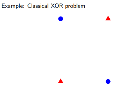
• Perceptron is very simple function while tasks in real world are very complex and connot be solved using it.

SUMMARY: Perceptron was proposed by F. Rosenblatt which was inspired by brain. Perceptron learns optimal weights corresponding to a hyperplane that seperates data into two classes, used for binary classfication. Perceptron prediction rule = \(\langle w, x \rangle > \theta\). While training perceptron we update perceptron weights to learn the seperating hyperplane. Weights updation rule when mistake occurs = \(w^{t+1} = w^t + x^ty^t\) . Perceptron will converge in finite steps as mistake bound for perceptron = \(M \leq \frac{\| w \|_2^2R^2}{\gamma^2}\) as number of mistakes are bounded so training is also bounded and it will converge in some finite steps. Perceptron only works when data is linearly seperable, and is not useful to learn complex boundaries.

References

• IE643- Deep Learning theory and practice in IIT Bombay taught by Prof. P. Balamurugan